

How an AI Token Travels Through a Data Center
Trace one prompt from gateway to scheduler, KV cache, GPU, and network — every component that powers AI inference.

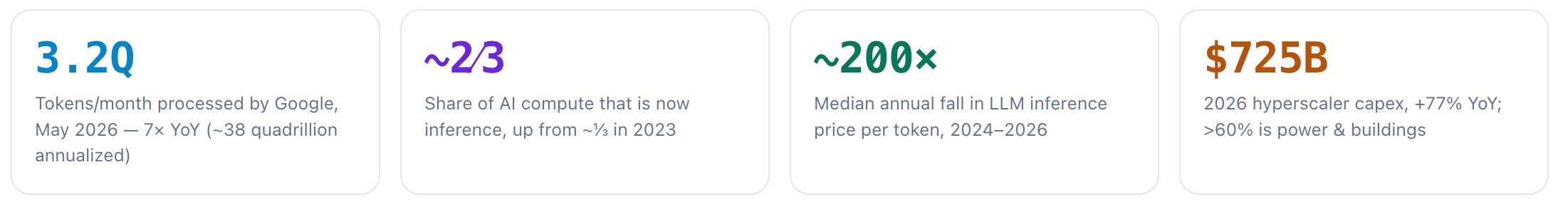
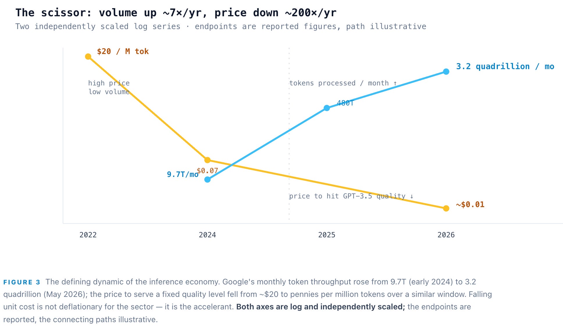
Every AI product you have ever used is, mechanically, the same object: a token generator. Strip away the branding and a chatbot, a coding agent, a search summary, and an image caption are all the identical operation — a trained model run forward to predict the next token, then the next, then the next. That operation is inference, and in 2026 it stopped being a footnote to training and became the entire game. In May 2026 Google disclosed it was processing 3.2 quadrillion tokens per month across its surface area — roughly 38 quadrillion tokens annualized — a 7× increase from 480 trillion a month a year earlier, which was itself up from 9.7 trillion in early 2024. None of that is training. It is the cost of answering.
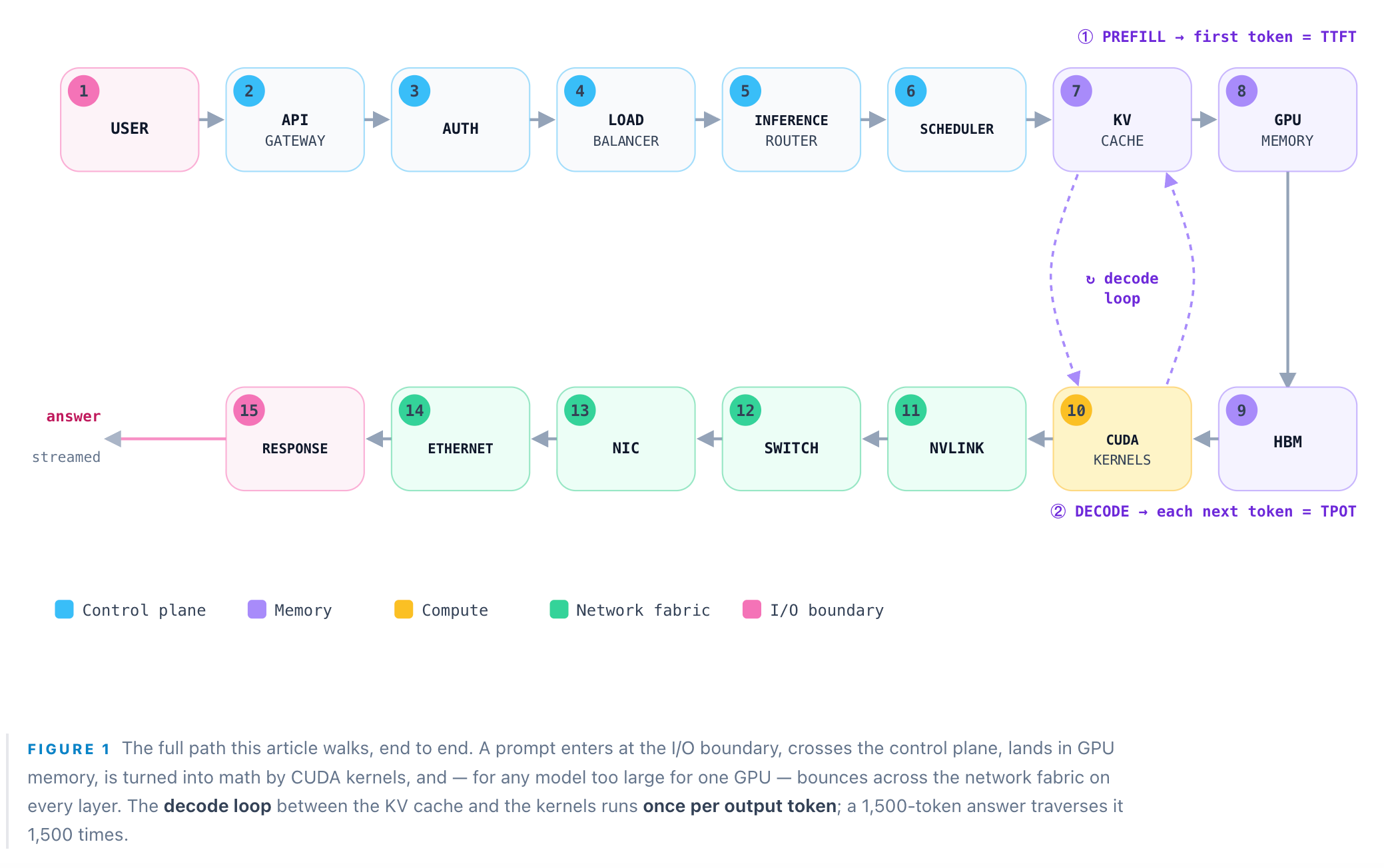
And yet inference is still treated as a black box: a prompt goes in, an answer comes out, a GPU is invoked somewhere in between. This piece opens the box. We take exactly one prompt and follow it literally — through fifteen physical and logical stops inside a datacenter — and explain precisely what each one does. By the end, “AI infrastructure” should stop being an abstraction and become something you can latency-budget, cost per token, and invest against.
The stakes behind that single round trip are the largest capital reallocation in the history of computing. Inference crossed roughly two-thirds of all AI compute in 2026, up from about one-third in 2023 and one-half in 2025. The four largest hyperscalers guided to ~$725B of 2026 capex, up 77% year over year, more than 60% of it going to power, cooling, and shells rather than chips. The market for inference-specific silicon alone will clear $50B in 2026. The single unit that ties this entire economy together is the token — and the token’s price is falling ~200× per year even as volume grows 7× per year. That scissor is the whole story: demand outruns a cost collapse, which is exactly the condition that turns an input into an economy.
The argument in five points
Inference is now roughly two-thirds of AI compute and 80–90% of a model’s lifetime cost. The token, not the model, is the unit of economic output.
Two phases, two bottlenecks: prefill is compute-bound (sets time-to-first-token) and decode is memory-bandwidth-bound (sets speed and cost). Nearly every optimization targets one of them.
Unit cost is falling ~200×/year while volume grows ~7×/year — Jevons, not deflation. “Enormous” and “high-margin” are different claims.
Durable value sits at the physical bottlenecks — memory bandwidth, scale-up interconnect, optics, and power. The inference-software layer is a real but contested business.
Buying inference is a weighted trade — latency (TTFT + speed + p99), blended cost, reliability (including the functional-availability gap), security, deployment, model coverage, and portability — scored against your workload.
The machine the economy runs on
The reason to care about the plumbing is economics. Training a model is a capital event — a one-time burn that produces a fixed asset. Inference is the cost of goods sold: it recurs on every query, forever, and it scales linearly with usage. The industry rule of thumb is that inference eventually accounts for 80–90% of the lifetime compute cost of a deployed model. So the shift in Figure 2 — inference passing from a third of compute in 2023 to two-thirds in 2026 — is not a fashion. It is the system reaching steady state, where most of the world’s accelerators spend most of their time serving, not learning.
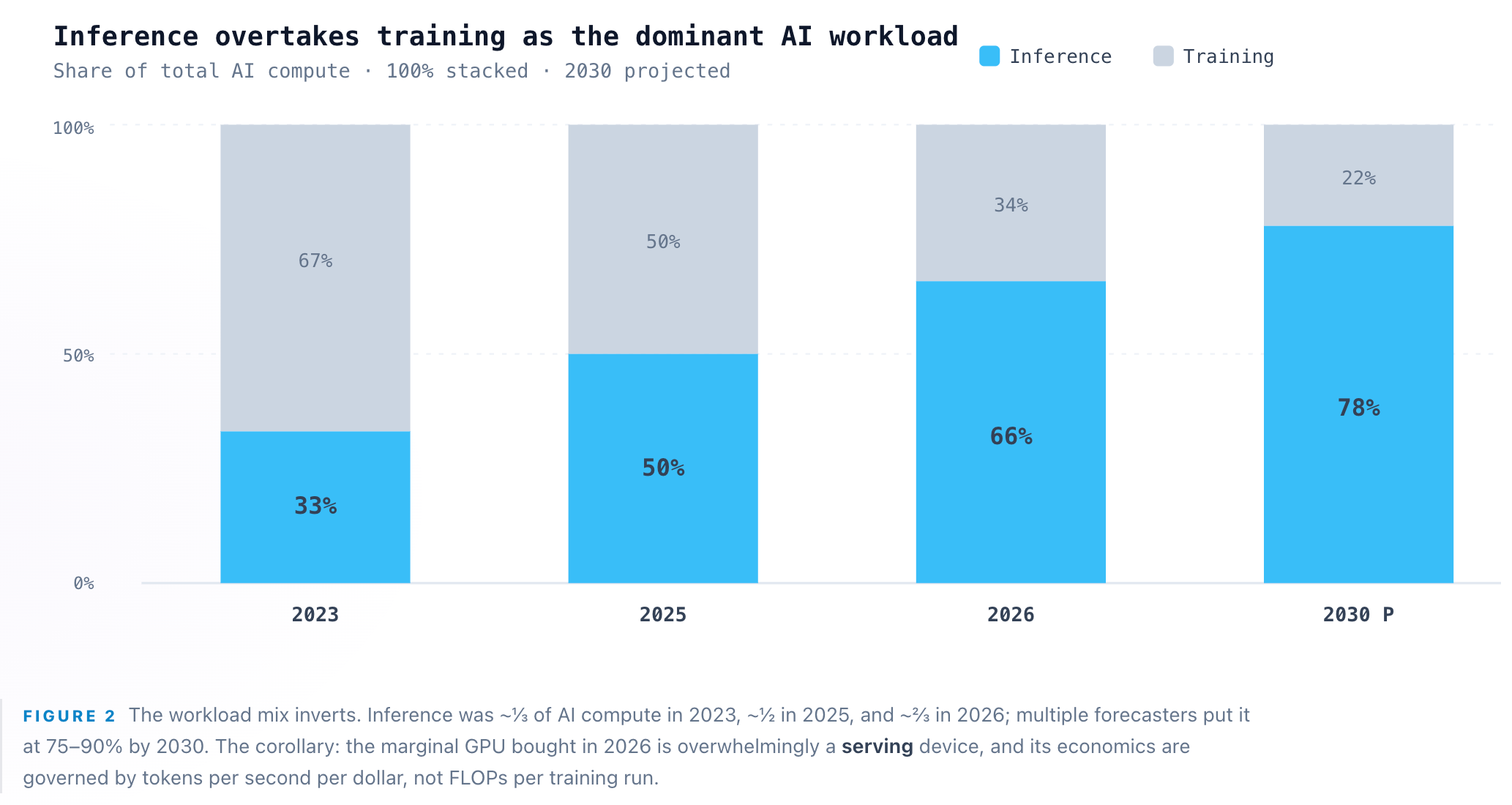
Two forces make this the defining infrastructure market of the decade. The first is that the frontier moved from bigger models to longer thinking: reasoning and agentic systems spend 10–100× more tokens per query. DeepSeek-R1 matched OpenAI’s o1 while emitting an order of magnitude more tokens per answer; agentic workflows — with their retries, tool calls, and context reloads — run 5–25× more expensive per task than a single-shot completion. The second force is a price collapse without modern precedent: the cost to serve a fixed quality level has fallen at a median ~200× per year since early 2024. Cheaper tokens do not reduce spend; they unlock new workloads faster than price falls. That is the Jevons paradox, and Figure 3 is what it looks like.
So the rest of this article is a single claim, made concrete: every technique below — batching, paging, quantization, speculation, disaggregation, and the network fabric itself — exists to move one number, cost per token at a target latency. Follow the specimen prompt and you will see exactly where each fraction of a cent and each millisecond is won or lost. Fifteen stops. Here is the first.
Step 1: User — the prompt becomes numbers
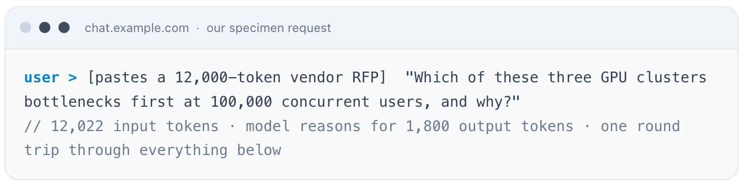
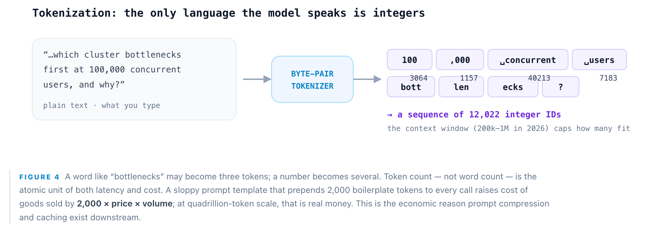
The journey begins before the datacenter. When you press enter, your client sends text over HTTPS — but the model never sees text. It sees integers. A tokenizer (a byte-level byte-pair encoder) chops the string into sub-word tokens, each mapped to an ID drawn from a vocabulary of roughly 100k–200k entries. Our 12,000-token RFP plus its question becomes a flat sequence of 12,022 integer IDs. Tokenization is deterministic, CPU-side, and effectively free — but it defines the bill. You are charged per token in and per token out, and the model’s context window (200k–1M tokens on 2026 frontier models) is a hard ceiling on how much of that RFP can enter at all.
Step 2: API Gateway — the front door
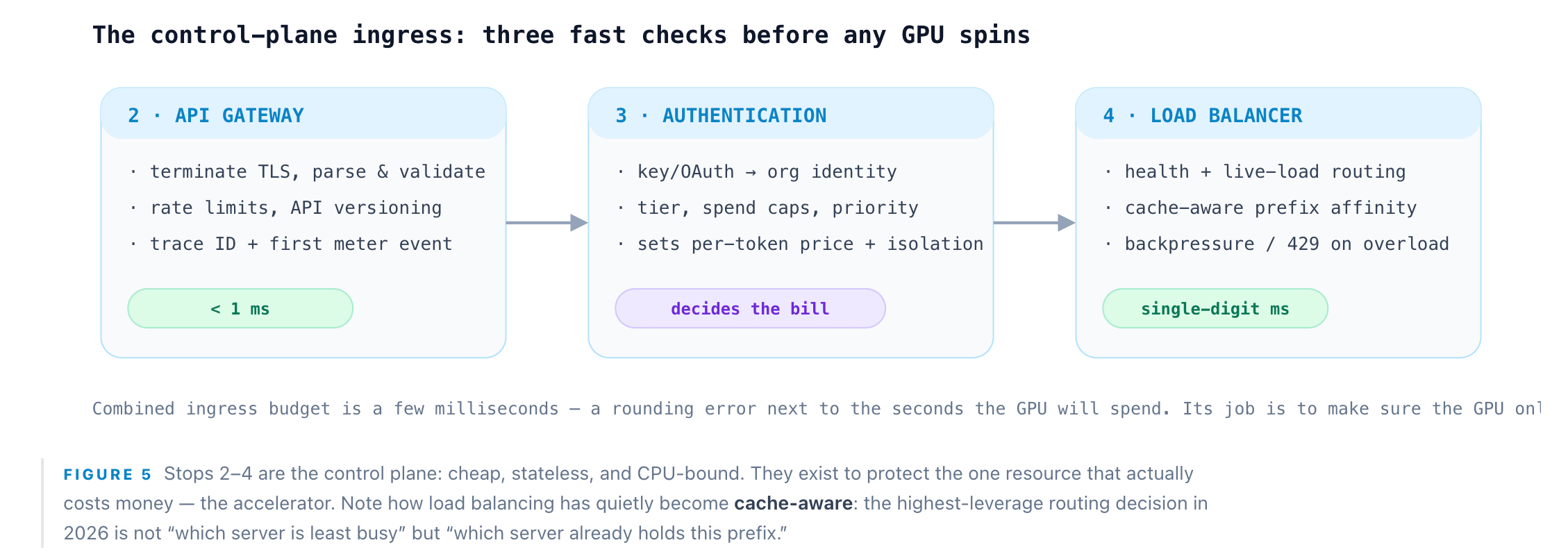
The request — still just an HTTPS body carrying those IDs — hits the API gateway, the datacenter’s front door. It terminates TLS, parses and validates the request against a schema, enforces API versioning, applies coarse rate limits, attaches a trace ID, and emits the first metering event. It is deliberately dumb and brutally fast: no model logic, just admission and bookkeeping at millions of requests per second, typically on Envoy- or NGINX-class proxies fronted by a web-application firewall. Latency budget: sub-millisecond. Its job is to reject the 5% of traffic that is malformed, over-quota, or hostile before any expensive resource is touched.
Step 3: Authentication — identity, tier, and the meter
Before a single GPU is touched, the request must be attributed. Authentication resolves the API key or OAuth token to an organization, checks its rate-limit tier and spend caps, and decides billing — the per-token price that will apply, whether the caller is eligible for cached-input discounts (a 50–90% reduction we will meet at stop 7), priority lanes, or cheaper batch pricing. It is also the security boundary: org-level data isolation and abuse defense. This stop is where a request stops being anonymous bytes and becomes a metered, priced, and isolated unit of work.
Step 4: Load Balancer — placing the request
Now the work must be placed on hardware. A conventional load balancer spreads requests across many identical model replicas using health checks and live load signals. But for LLM serving, naive round-robin is actively wasteful: two requests that share a long prefix — the same system prompt, the same pasted RFP — should ideally land on the same replica so the expensive prefix computation can be reused from cache. So modern AI load balancing is becoming cache-aware, which is exactly why it blurs into the inference router at the next stop. The load balancer also enforces backpressure: when the fleet is saturated, it is the component that decides whether you queue or get a 429.
Step 5: Inference Router — model, silicon, and kernel selection
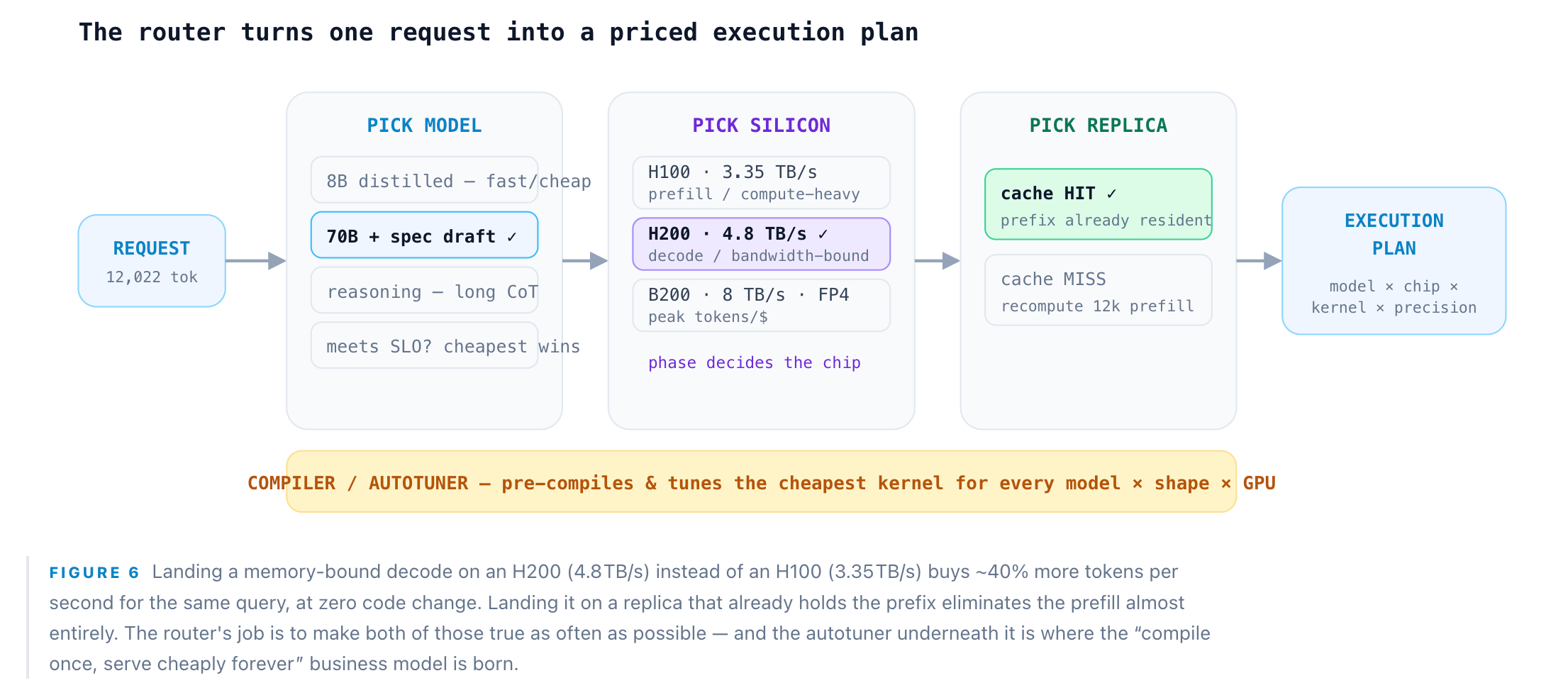
The router is where inference gets interesting, and where a startling amount of gross margin is won or lost. In a few milliseconds it answers three questions. Which model? A frontier 70B, a distilled 8B, a reasoning variant, or a speculative draft + target pair — serving a query on a 70B when an 8B meets the service-level objective is pure margin destruction. Which silicon? This is hardware selection, and it is phase-dependent: the compute-bound prefill wants raw FLOPs, while the memory-bound decode wants HBM bandwidth, so the “right” GPU differs within a single request. Which replica? Cache-aware routing sends the request to the instance that already holds this prefix’s KV cache, converting a 12,000-token prefill into a near-free cache hit.
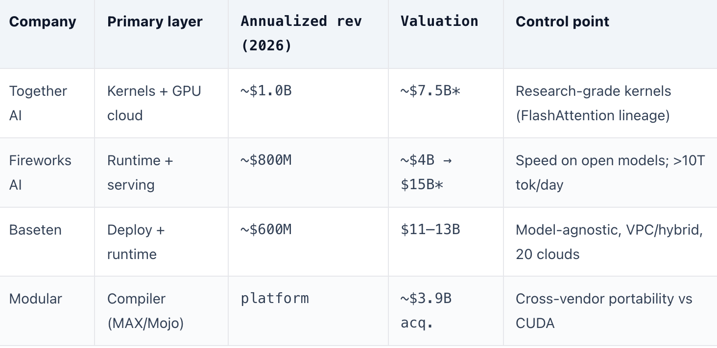
This stop is also home to the compiler / autotuner layer — the systems that, ahead of time, compile and tune the exact GPU kernels for a given model, shape, and chip, and at runtime select the cheapest execution plan. This is not academic: it is a business. Together AI, Fireworks, Baseten, and Modular were each built, in large part, at this layer — turning “which kernel on which chip at which precision” into a product, then monetizing it with their own inference infrastructure. We return to that model, and its valuations, at the end of the journey.
Step 6: Scheduler — the batching engine that funds it all
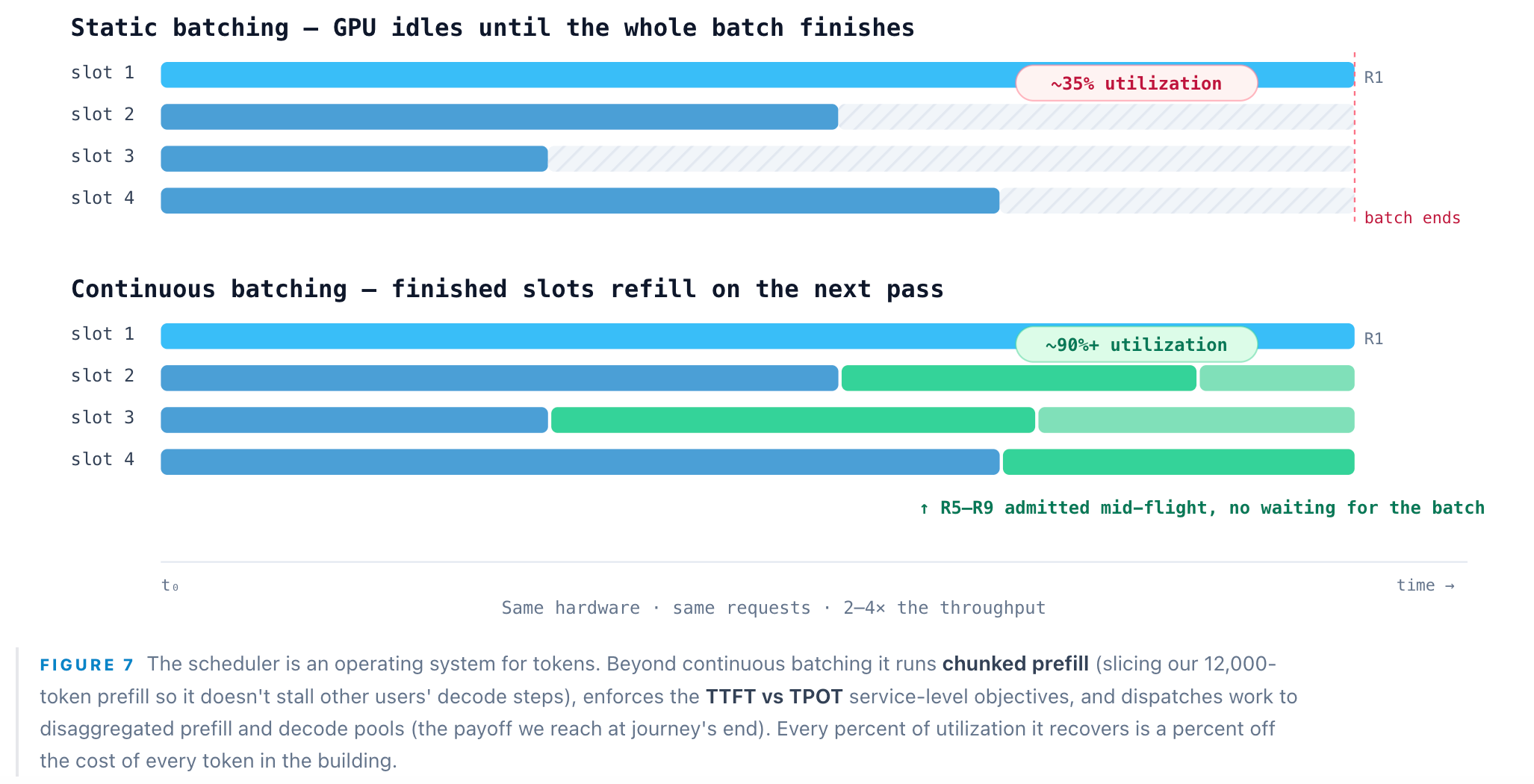
If a single component makes GPU economics work, it is the scheduler. A lone decode step underuses a GPU catastrophically: at batch size 1, an H100 runs at roughly 30–40% streaming-multiprocessor utilization because it is starved on memory, not math. The scheduler’s answer is continuous (iteration-level) batching: rather than fixed batches, it interleaves many sequences and, at every forward pass, admits freshly-arrived requests and evicts finished ones, keeping the GPU saturated pass after pass. This one trick is the core of vLLM, which delivers 2–4× the throughput of prior serving systems and 3–5× the traffic of a naive PyTorch loop on the same H100.
Step 7: KV Cache — the memory that makes generation possible
Now the request is on a GPU, and we hit the single most important data structure in inference. Inside every attention layer, each token produces a Key and a Value vector. To generate token N+1, the model must attend to the K and V of every prior token — so recomputing them at each step would cost O(n²) and be ruinous at a 12,000-token context. Instead they are cached: the KV cache. Prefill computes and stores K/V for all 12,022 positions once; each subsequent decode step appends one token’s K/V and reads the rest. The KV cache is the largest and most dynamic consumer of GPU memory during serving, and managing it well is most of what a modern inference engine does.
The hard part is fragmentation. Sequences grow to unpredictable lengths, and classic contiguous allocation strands 60–80% of memory. vLLM’s PagedAttention borrows the operating-system trick of virtual memory: the KV cache is split into fixed-size blocks (“pages”), allocated on demand and mapped through a page table, so physical blocks need not be contiguous and finished sequences free their pages instantly. That is the mechanism behind vLLM’s 2–4× throughput — and it is what lets many users’ sequences safely share one GPU.
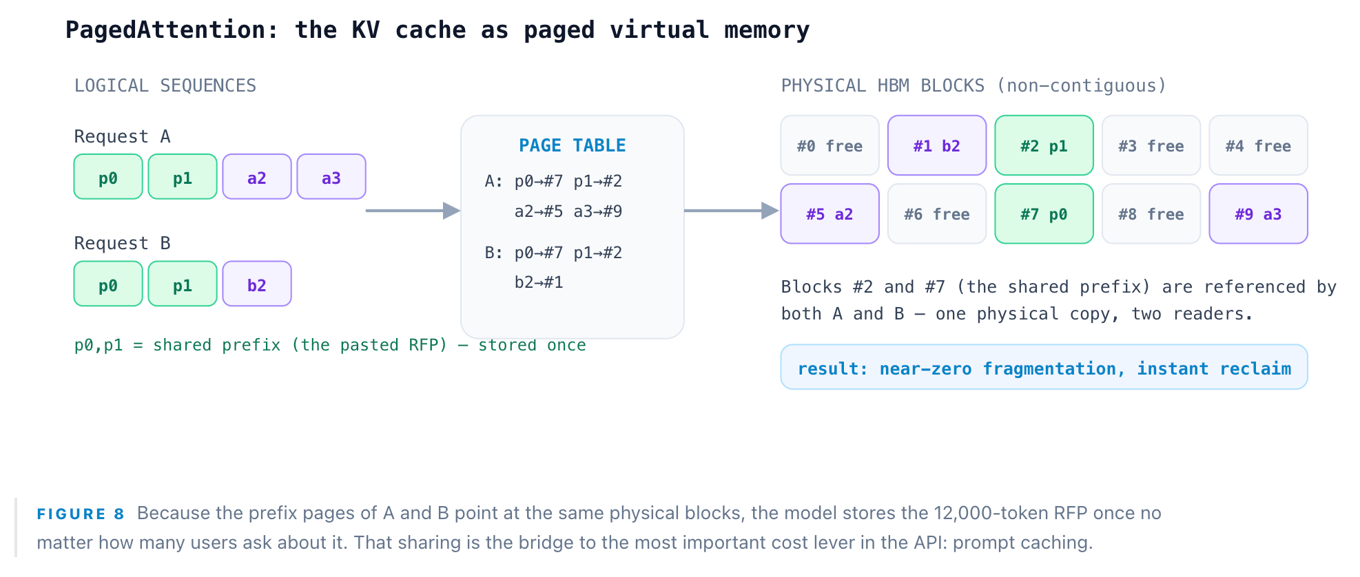
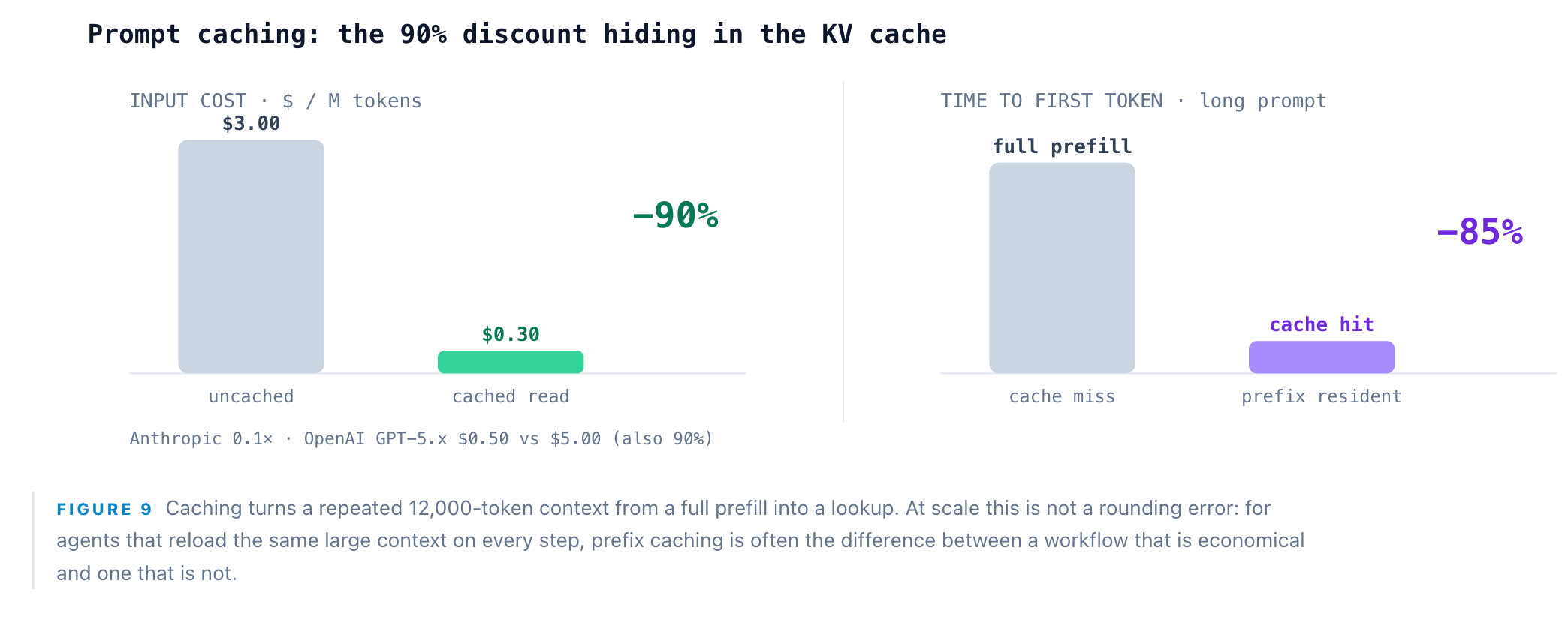
That sharing is not just a memory optimization — it is a price. If many requests carry the same prefix (a system prompt, a long few-shot preamble, our pasted RFP), its KV cache can be computed once and reused across calls. Providers now sell this directly as prompt / prefix caching: Anthropic charges cached reads at 0.1× input ($0.30 vs $3.00 per million tokens); OpenAI’s GPT-5.x line prices cached input at $0.50 vs $5.00 — both a 90% discount, with roughly 85% lower latency on long prompts. For our specimen, caching the RFP collapses a 12,022-token prefill into a near-free cache hit on every follow-up question.
Step 8: GPU Memory — the real constraint on who you can serve
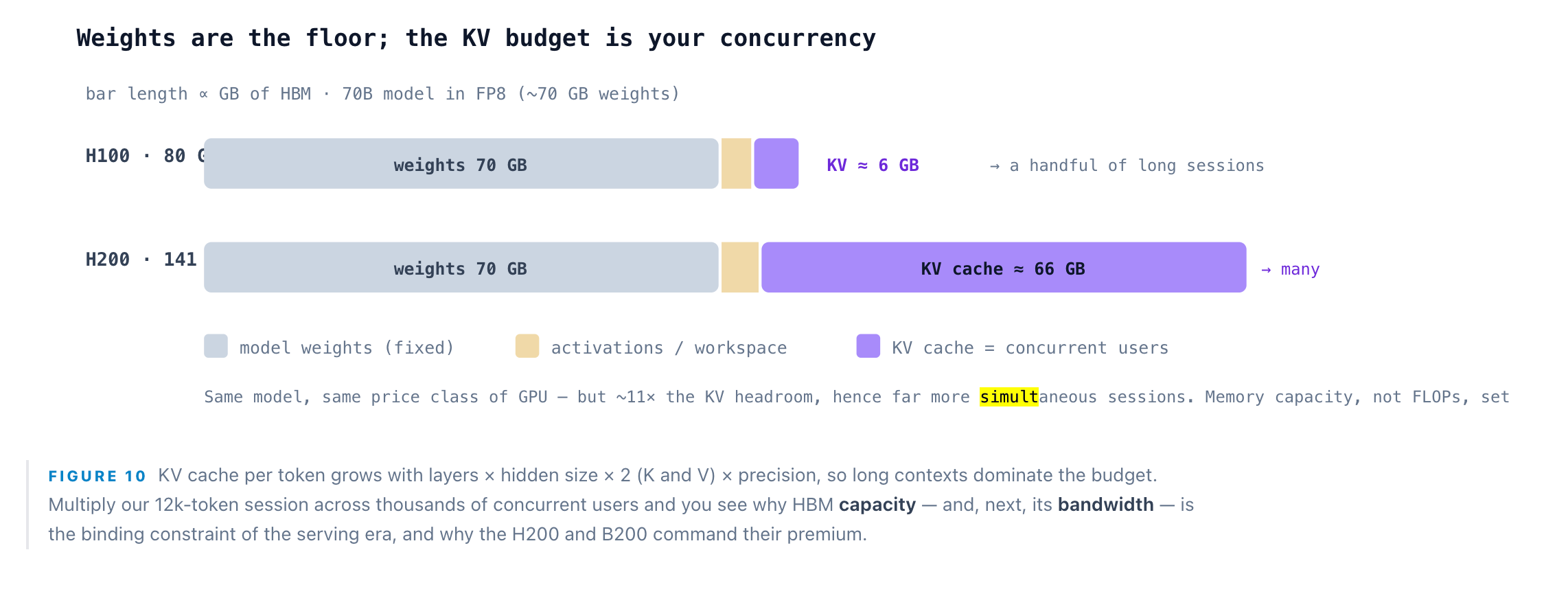
A serving GPU’s on-package memory holds three things at once: the model weights (fixed), the KV cache (grows with the number of concurrent sequences and their length), and activations and workspace (transient). The weights are the floor; whatever remains is the KV budget, and that budget — not compute — usually caps concurrency. A 70B model is ~140 GB in FP16 and needs two 80 GB H100s just to load; in FP8 it is ~70 GB and fits one GPU with room left for KV cache. This is the first place quantization pays for itself: every gigabyte shaved off the weights becomes KV headroom, and KV headroom is the number of users you can serve simultaneously.
Step 9: HBM — the bandwidth wall and the roofline
This is the counterintuitive heart of the whole machine. Prefill and decode stress entirely different resources. Prefill processes all 12,022 input tokens in parallel — one enormous matrix multiply that saturates the tensor cores. It is compute-bound, and it sets TTFT. Decode is the opposite: to produce each single next token, the GPU must stream the model’s entire weight tensor (plus the growing KV cache) out of HBM, once per token. That read time is fixed by memory bandwidth, not math. At batch size 1, decode’s arithmetic intensity is about 1 FLOP per byte — far below the roofline’s ridge point of ~410–590 FLOP/byte — so the tensor cores sit almost entirely idle, waiting on memory.
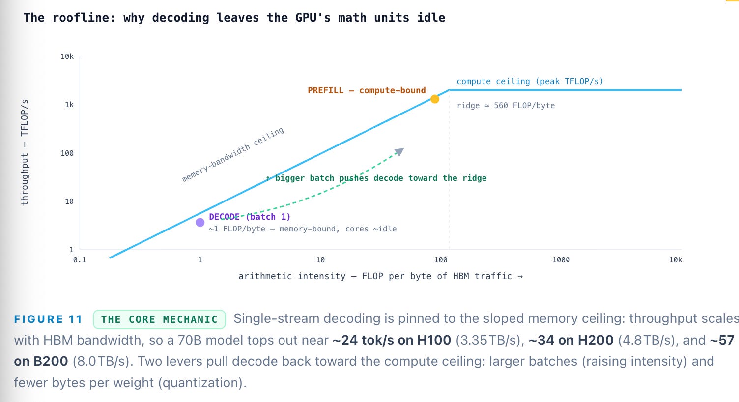
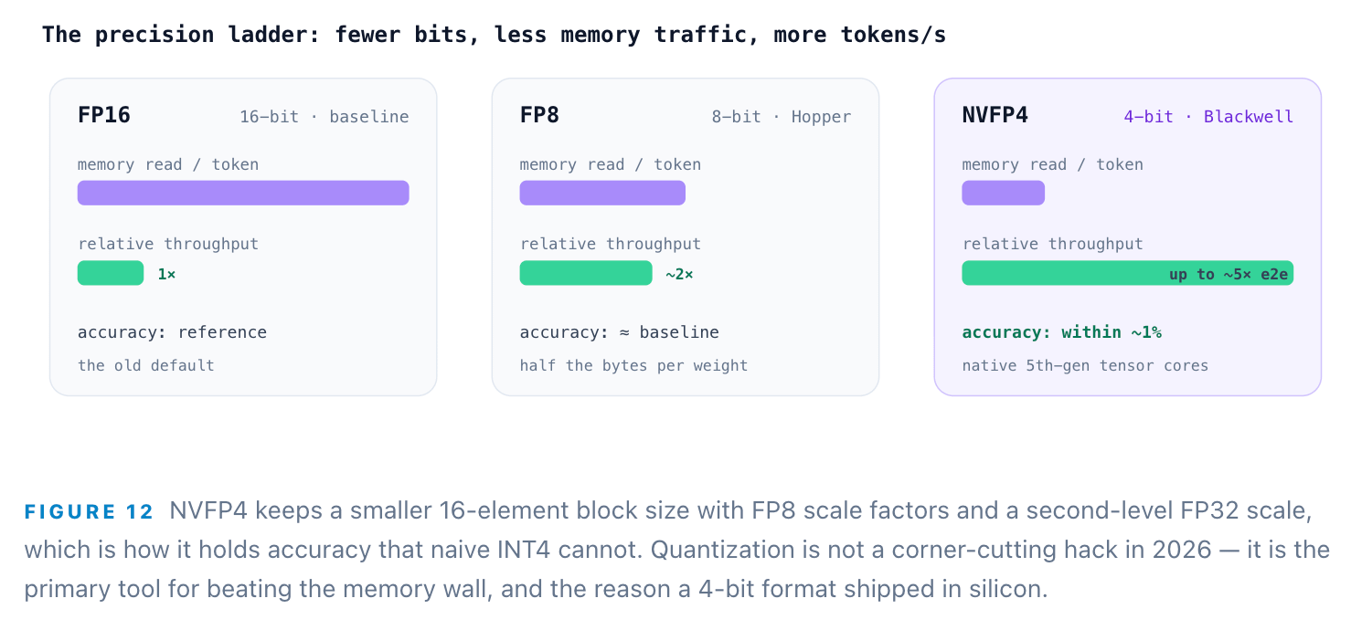
So the industry is marching down the precision ladder: FP16 → FP8 → FP4. Fewer bits per weight means fewer bytes to read per token, which directly lifts the memory-bound decode ceiling. NVIDIA’s NVFP4 — a 4-bit floating-point format native to Blackwell’s 5th-generation tensor cores — delivers roughly 2–3× the arithmetic throughput of FP8 and ~1.8× memory reduction while holding within about 1% of baseline accuracy, contributing to end-to-end inference speedups up to 5× versus Hopper. Every bit dropped is bandwidth reclaimed and a token made cheaper — the single most direct lever on cost of goods sold in the building.
Prefill is compute-bound and sets your time-to-first-token; decode is memory-bandwidth-bound and sets your speed and cost. Nearly every technique in inference is an attack on that decode memory wall — batch bigger, quantize smaller, speculate ahead. Read: Why KV Cache and Memory Drive AI Economics.
Step 10: CUDA Kernels — where tokens become arithmetic
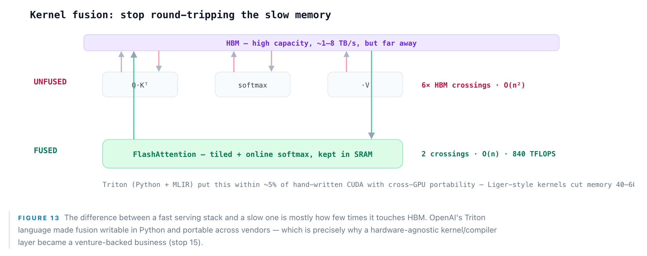
The execution plan is now math, and math on a GPU runs as kernels — small programs executed across thousands of cores. The naive way to run a transformer is hundreds of separate kernel launches, each reading its inputs from HBM, computing, and writing results back. For a bandwidth-bound workload that round-tripping is fatal. So the entire craft is kernel fusion: collapse many operations into one kernel that keeps intermediate data in fast on-chip SRAM and touches slow HBM as little as possible. The canonical example is FlashAttention, which computes attention in tiles with an online softmax, cutting HBM reads and writes from quadratic to linear in sequence length for 2–4× speedups. FlashAttention-3 exploits Hopper’s asynchronous engines and FP8 to reach 840 TFLOPS on an H100 — about 85% of peak.
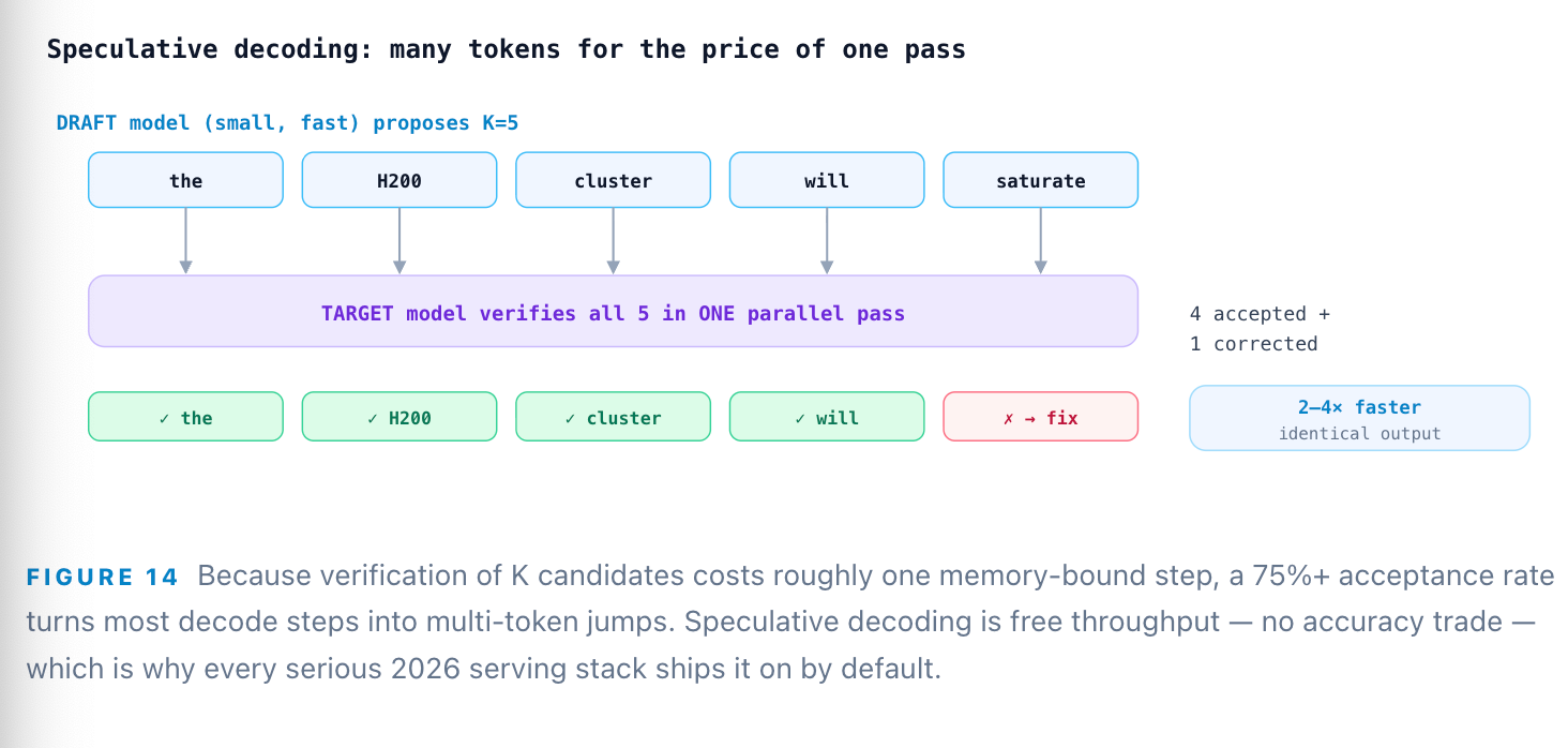
One kernel-level trick deserves its own spotlight because it is the highest-ROI optimization in single-stream serving: speculative decoding. Since decode is memory-bound — the GPU reads all the weights per step no matter what — you can verify several candidate tokens for almost the same cost as generating one. A small, cheap draft model proposes the next K tokens; the large target model checks them all in a single parallel pass and accepts the longest correct prefix. The output is mathematically identical to ordinary decoding, but 2–4× faster. Modern methods like EAGLE-3 push draft acceptance rates above 75%.
Step 11: NVLink — when one GPU is not enough
Our 70B specimen fits on a single GPU, but the frontier does not: trillion-parameter and mixture-of-experts models are sharded across many GPUs, which means the GPUs must talk to each other — on every layer, for every token. This is the point people miss: networking sits directly inside the decode loop, not off to the side. The first fabric is scale-up — NVLink — the ultra-fast interconnect that fuses many GPUs inside a rack into one logical accelerator. NVLink 5 moves 1.8 TB/s per GPU, about 14× a PCIe Gen5 link. The GB200 NVL72 wires 72 Blackwell GPUs and 36 Grace CPUs into a single NVLink domain with 130 TB/s aggregate bandwidth and 13.4 TB of unified memory — one rack behaving as one machine, delivering up to 30× the inference throughput of an H100 cluster on trillion-parameter models, while drawing ~120 kW.
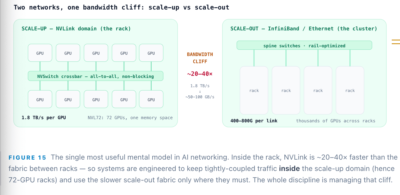
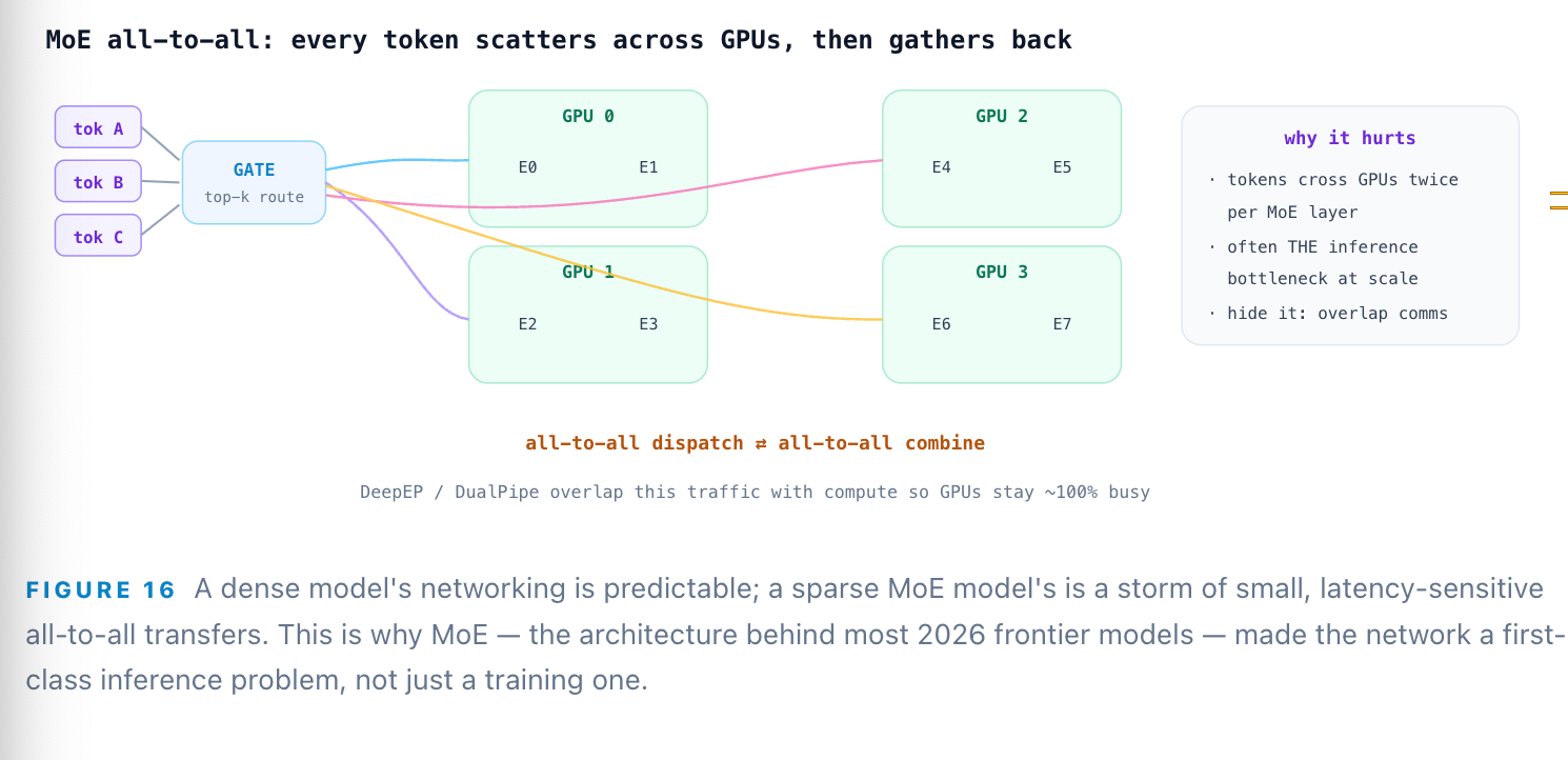
Why is such extreme bandwidth necessary? Because parallelism creates traffic. Tensor parallelism splits each layer’s matmul across GPUs, and after every one the partial results must be summed with an all-reduce collective — many times per token. Worse, mixture-of-experts models route each token to a handful of experts scattered across GPUs, triggering all-to-all communication that frequently becomes the dominant inference bottleneck. DeepSeek’s production stack uses eight 400 Gbps NICs per node and a bespoke library (DeepEP) to overlap this exchange with computation so the GPUs never stall.
Step 12: Switch — the crossbar and the congestion problem
A fabric needs switches. Inside the scale-up domain, NVSwitch is the crossbar: 144 NVLink ports and 14.4 TB/s of non-blocking switching, so all 72 GPUs can talk at full speed at once. Beyond the rack, the scale-out network uses its own switches — NVIDIA’s Quantum-X800 (InfiniBand) and Spectrum-X800 (Ethernet), or Broadcom’s Tomahawk 6 at 102.4 Tbps (64 × 1.6T ports). Two things make an AI switch unlike a cloud switch. First, rail-optimized topology: GPUs are cabled so that the n-th GPU in every server homes to the same “rail” switch, minimizing hops for collectives. Second, in-network computing and congestion control: switches can perform reductions in-fabric (SHARP), and they must absorb the synchronized “incast” of thousands of GPUs finishing a step at the same instant. One congested link stalls an entire collective — the tail-latency problem — so adaptive routing is existential, not optional.
Step 13: NIC — the GPU’s on-ramp to the cluster
A packet leaving the GPU for another rack goes through a network interface card — in 2026, almost always a SmartNIC or DPU (NVIDIA BlueField and peers). Its core job is RDMA over Converged Ethernet (RoCE) or InfiniBand verbs: letting a remote GPU read this GPU’s memory directly, bypassing both CPUs, at 400 Gb/s today and 800 Gb/s becoming standard. But the DPU is a full programmable computer on the NIC: it offloads congestion control, encryption, storage virtualization, and multi-tenant isolation from the host CPU. In a rail-optimized cluster each GPU typically owns a dedicated NIC — DeepSeek pairs eight GPUs with eight 400 Gb/s NICs — so no accelerator shares an on-ramp. This is where “the network” physically begins for a byte, and it is the boundary where our data-gravity theme becomes literal.
Step 14: Ethernet — the scale-out fabric, and the optics beneath it
Historically AI clusters ran on InfiniBand for its ~1–2 µs latency and lossless fabric; Ethernet with RoCEv2 sat at ~5–10 µs and was treated as second-tier for training. That hierarchy is inverting. The Ultra Ethernet Consortium shipped UEC 1.0 in June 2025 — a 560-plus-page rebuild of the Ethernet stack for AI — closing the latency and reliability gap, and Dell’Oro projects Ethernet overtakes InfiniBand in AI back-end networks by 2027. 800G is already the default port speed, with Broadcom’s Tomahawk 6 pushing 102.4 Tbps. For inference specifically — cost-sensitive, multi-tenant, enterprise-adjacent — Ethernet’s economics and open ecosystem are decisive.
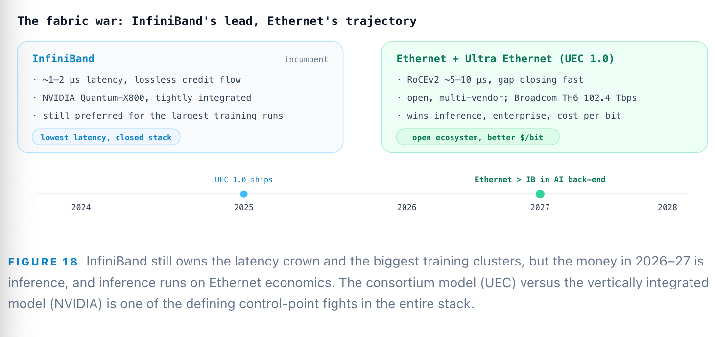
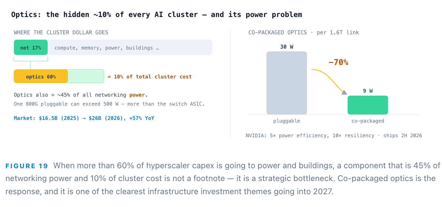
Underneath the fabric is its least-discussed cost center: optics. Optical transceivers are roughly 60% of networking cost and 45% of networking power; with networking at ~15–18% of total cluster cost, optics alone are close to 10% of the entire bill. A single 800G pluggable can burn more than 500 W across a switch — more than the switching ASIC itself. The AI optical-transceiver market is running from ~$16.5B in 2025 to ~$26B in 2026 (+57% YoY). The structural fix is co-packaged optics: move the optics onto the switch package, cutting a 1.6T link from ~30 W to ~9 W, with NVIDIA claiming 5× power efficiency and 10× resiliency for its photonics switches shipping in 2H 2026.
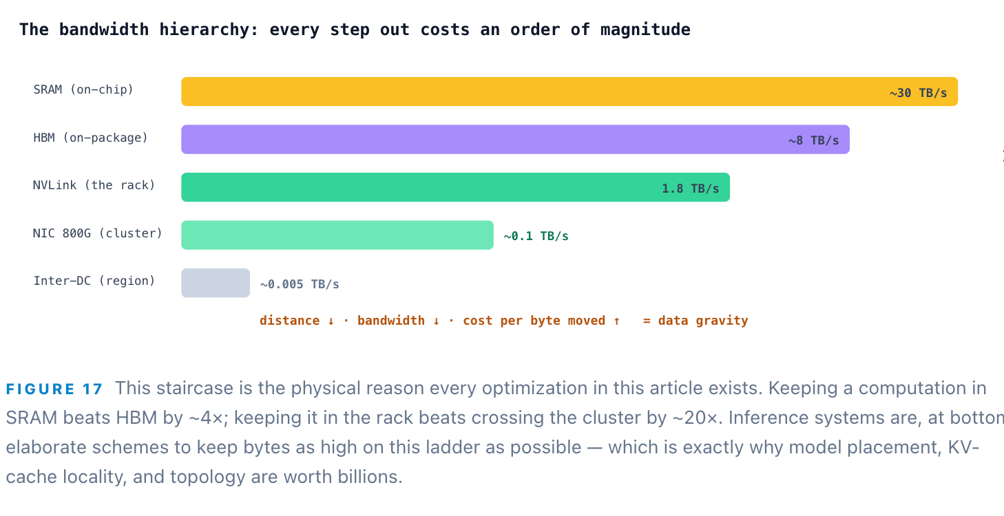
For any model too big for one GPU, the network sits inside the decode loop — it runs on every layer, every token. Managing the ~20–40× bandwidth cliff between scale-up (NVLink) and scale-out (Ethernet) is the whole game.
Step 15: Response — detokenize, stream, and settle the bill
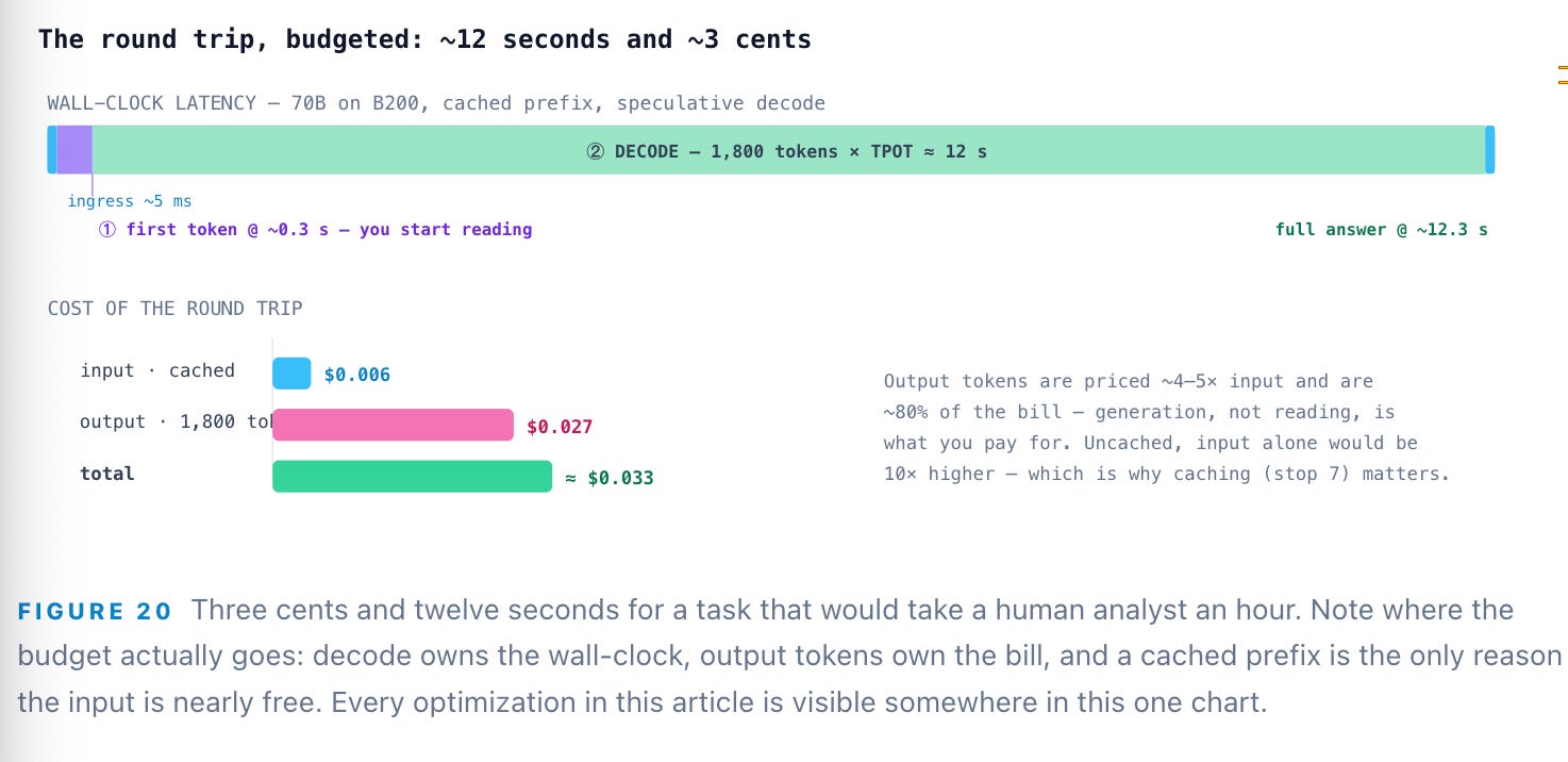
The last token is generated, and now the trip runs in reverse. Detokenization maps the integer IDs back into text, and the answer streams token-by-token back out through the NIC, the switch, the load balancer, and the gateway to the user — typically over server-sent events, so tokens appear as they are produced. This is why time-to-first-token dominates perceived speed: the user starts reading at ~0.3 s even though the full answer takes seconds to finish. The final act is the meter closing the bill — input tokens (possibly cached), output tokens (the expensive ones), priced at the tier that authentication assigned back at stop 3. Fifteen stops, one answer.
Final Step: Putting it together: the inference OS
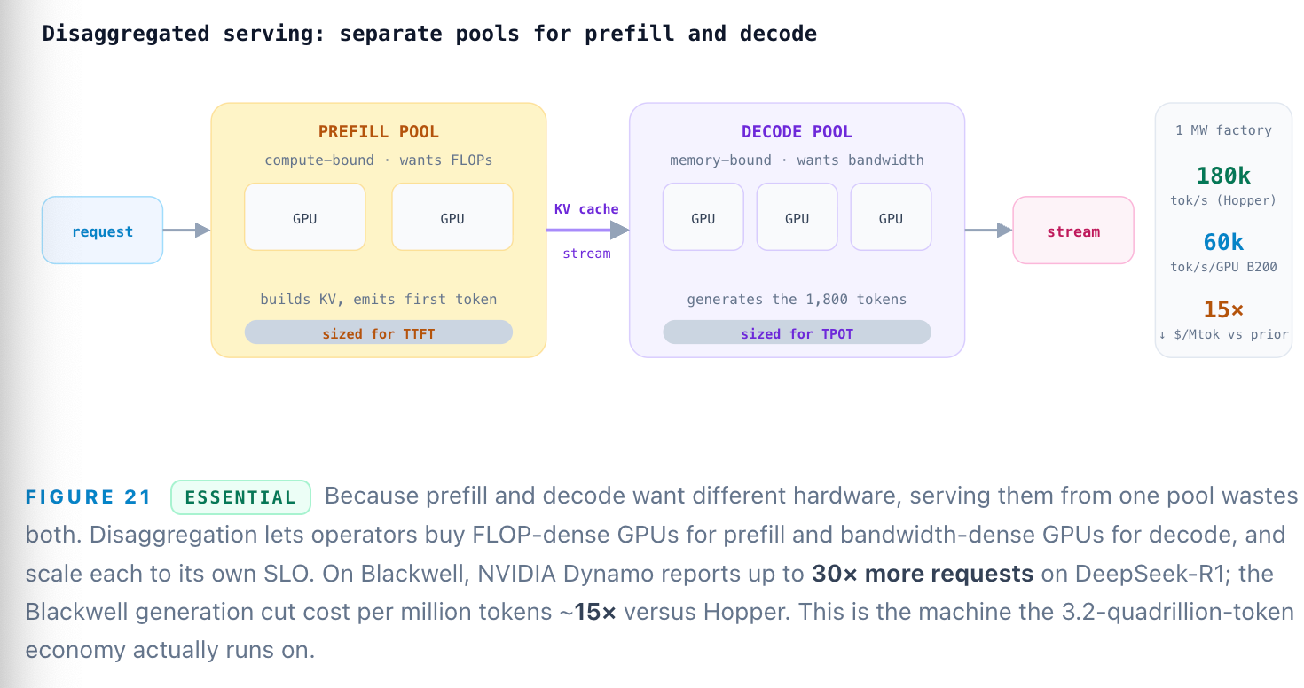
Walk the fifteen stops again and a pattern emerges: the hard problems — batching, KV paging, prefill vs decode, hardware selection, collective communication — are all really one problem, which is scheduling heterogeneous work across a memory-and-network hierarchy to keep expensive silicon saturated. The 2026 answer is disaggregated serving: split the compute-bound prefill and the memory-bound decode onto separate GPU pools, each scaled and tuned independently, and stream the KV cache between them. This is now standard across NVIDIA Dynamo, vLLM, SGLang, llm-d, and Mooncake.
The business of the stack: compilers that became clouds
The most interesting companies on this map sit at stops 5 and 10 — the compiler, kernel, and autotuner layer — and they discovered the same thing: the way to monetize a better kernel is not to license it, but to run it. Own the inference infrastructure, sell tokens, and keep the efficiency delta as gross margin. The logic is airtight. Every 2× you win in kernels, batching, quantization, or speculative decoding is 2× more tokens per GPU — and if you are the one operating the GPUs, that is margin you capture rather than a benchmark you publish. An autotuner that compiles the cheapest kernel for every model × shape × chip is, in effect, a money printer bolted to a fleet.
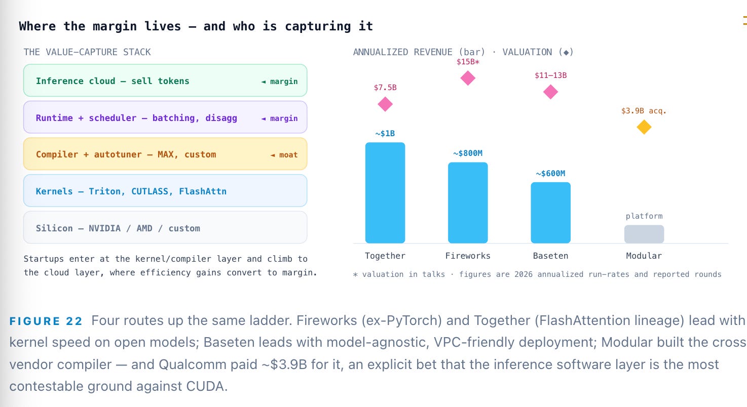
The growth rates are the argument. Baseten’s run-rate went from ~$200M (Dec 2025) to ~$600M by March 2026 — roughly 1,900% YoY — as it closed a $1.5B round at $11–13B, up from $5B five months earlier. And Modular’s ~$3.9B sale to Qualcomm is the clearest signal of all: a chipmaker buying a hardware-agnostic compiler to attack NVIDIA exactly where the moat is thinnest.
Choosing an inference provider: the real decision criteria
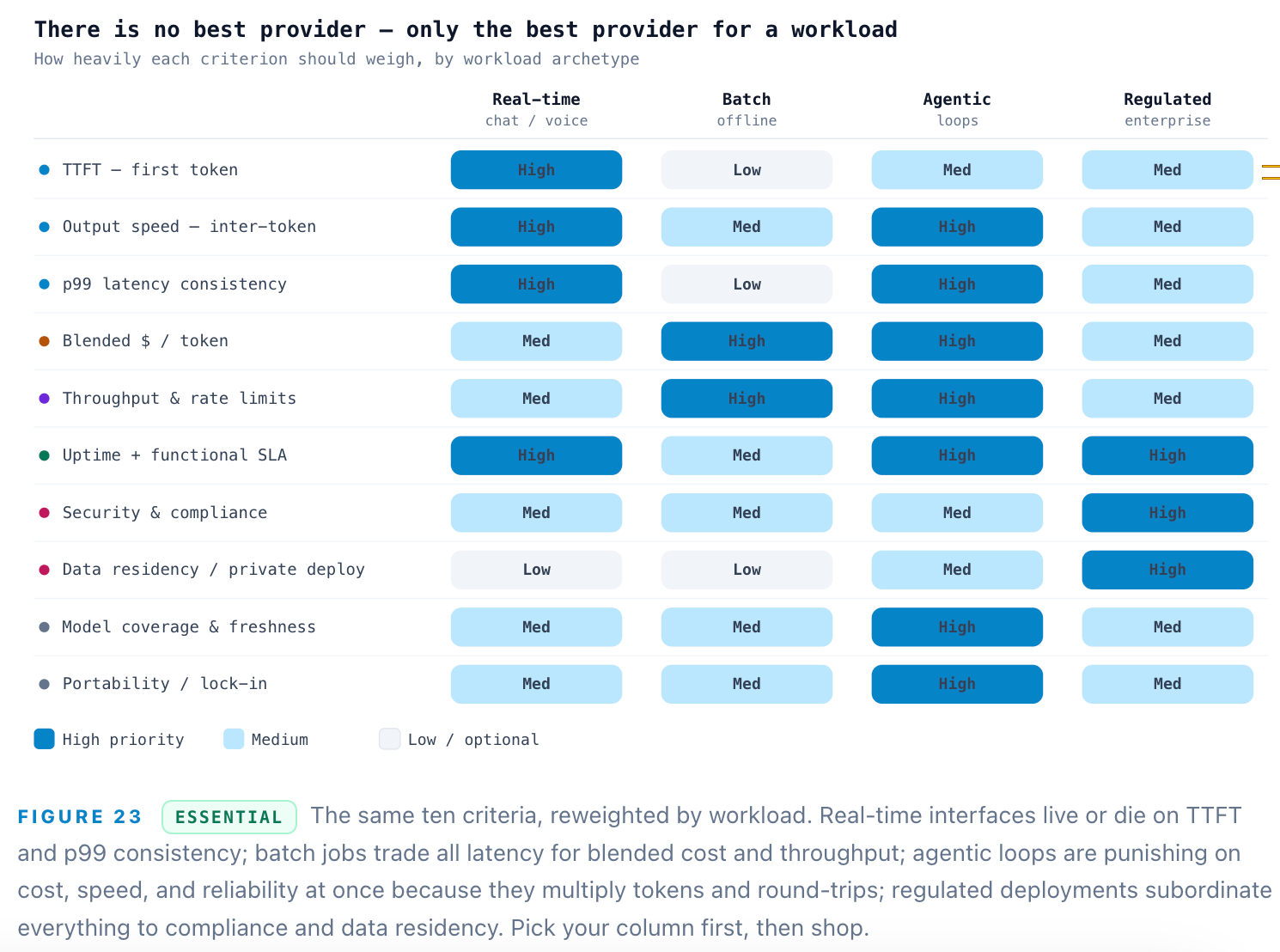
If you are buying inference rather than building it, the fifteen-stop machine collapses into a purchasing decision — and the most common mistake is optimizing for a headline price per million tokens. There is no best provider in the abstract; there is only the best provider for a workload shape. A real-time voice agent, a nightly batch summarizer, a multi-step autonomous agent, and a HIPAA-bound enterprise app weight the same criteria completely differently. The framework below is the one that survives contact with production.
The three everyone names — measured correctly
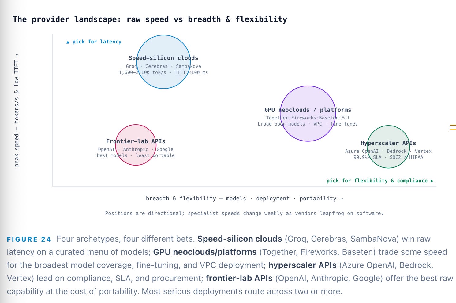
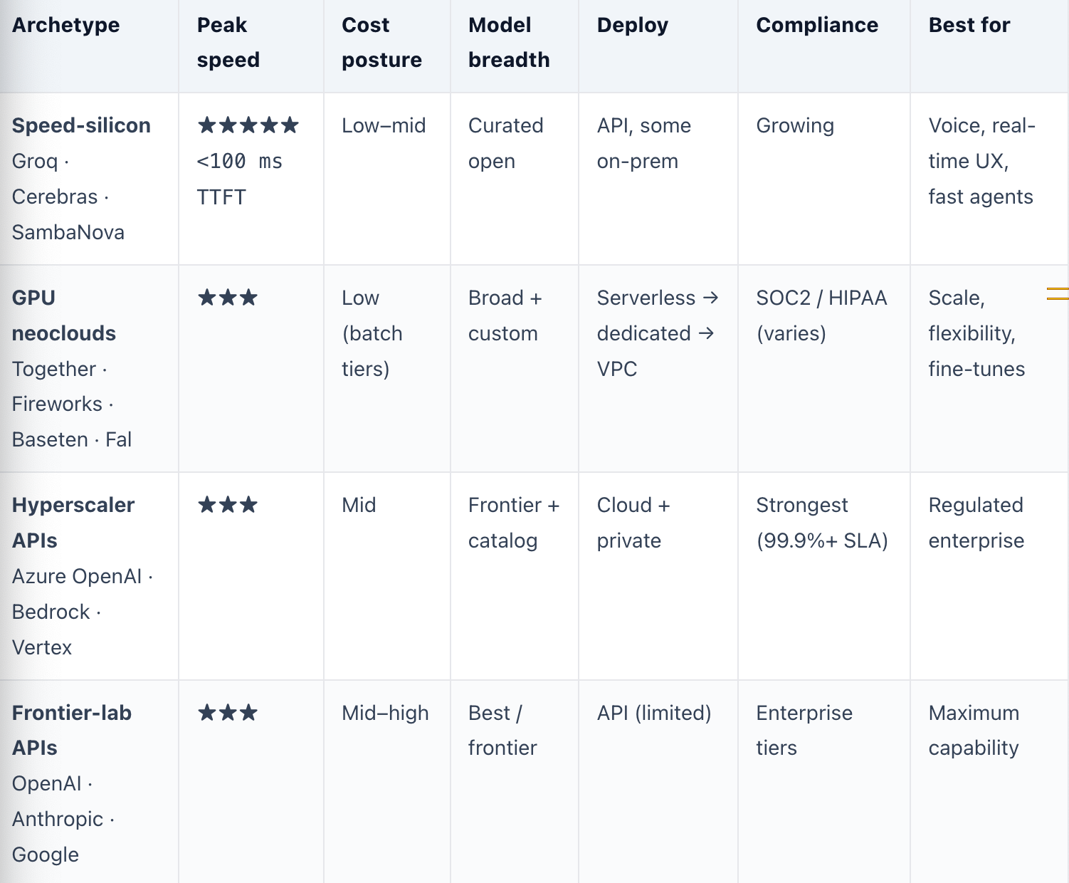
Latency is two numbers, not one. Time-to-first-token (the prefill latency) governs how fast the answer starts; inter-token latency, or output speed, governs how fast it finishes. A provider can win one and lose the other, and the number that matters for user experience is the p99 tail, not the median — a great p50 with a poor p99 still produces visible stalls. Typical GPU inference lands first tokens in ~400–600 ms; the speed-silicon clouds compress that sharply, with Groq and Cerebras posting sub-100–150 ms TTFT and output speeds of 1,600–2,100+ tokens/second on Llama-70B-class models — roughly 4–6× a typical GPU stack.
Cost is blended, not posted. The list price is two numbers — input and output per million tokens — and output is priced ~4–5× input and usually dominates. Your real unit cost depends on your input:output ratio, your cache-hit rate (prompt caching cuts input 50–90%), and whether the work can use a batch tier (often ~50% cheaper). Posted rates in mid-2026 span two orders of magnitude — from roughly $0.04–$0.20 per million on cost-optimized open-model endpoints (DeepInfra; Groq at $0.15/$0.60) to several dollars per million for frontier models — so two providers with identical headline prices can differ 3× on your traffic.
Reliability is more than an uptime percentage. The formal SLA (Azure OpenAI publishes 99.9% for token generation; enterprises increasingly demand a latency SLA such as sub-200 ms TTFT for 99.99% of calls) is necessary but not sufficient. The failure modes that actually break products sit outside it: refusal spikes, silent model-version bumps that regress your evals, and quota-driven throttling under load. A vendor can honor 99.95% uptime and still degrade your application through any of these — which is why the mature answer is to pin model versions, negotiate capacity, and monitor functional availability yourself.
The seven everyone forgets
Beyond latency, cost, and reliability, seven criteria decide production fit. Throughput & rate limits (tokens-per-minute ceilings and burst headroom) gate agentic fan-out and scale. Security & compliance — SOC 2 Type II, HIPAA, ISO 27001, GDPR — is table stakes in regulated industries and slow to retrofit. Data residency & private deployment (zero-retention guarantees, VPC/BYOC, on-prem) is what clears enterprise procurement; most consumer-grade endpoints leave retention vague and offer no private path, quietly disqualifying themselves. Determinism & version control — fixed seeds, pinned checkpoints — protects your evaluation suite from silent drift. Model coverage & freshness (breadth, day-zero support for new open weights, fine-tune/LoRA hosting) sets how fast you adopt the frontier. Deployment flexibility (serverless vs dedicated vs self-host) sets your cost/control trade. And portability — an OpenAI-compatible API and clean multi-provider routing — is your insurance against every one of the above going wrong.
Pick your workload column first, then shop. A headline price per million tokens is close to meaningless without your input:output ratio, your cache-hit rate, and a latency SLA that covers the p99 tail.
The reliability trap most teams learn the hard way
A provider’s 99.95% uptime does not cover the failures that actually page you: a silent model swap that tanks your eval scores, a refusal-rate spike after a safety update, or quota throttling exactly when traffic peaks. Treat the SLA as a floor, pin model versions, and monitor functional availability yourself.
Implications: where the value accruescore
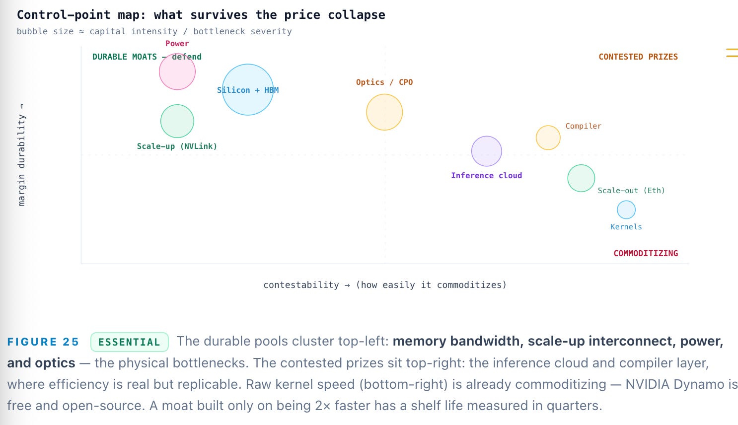
Three conclusions follow. First, the physical bottlenecks compound: HBM bandwidth sets the decode ceiling, the NVLink scale-up domain is genuinely proprietary, and optics plus power are the scarce inputs — more than 60% of that $725B capex is already power and buildings, which makes tokens per watt the terminal metric. Second, the network is bifurcating: scale-up stays closed and defensible while scale-out goes open (Ethernet/UEC) and commoditizes, so the edge is the scale-up domain, optics/CPO, and congestion IP — not commodity switching. Third, the inference-software layer is real but contested: margin equals efficiency delta × utilization × scale, durable only where a player has converted speed into distribution and switching costs before the price collapse makes raw performance table stakes.
The decisive read: through 2027, back the bottlenecks — memory and bandwidth, scale-up interconnect, optics and power — and the inference platforms that have already turned efficiency into lock-in. Be skeptical of anything whose entire pitch is raw speed, because raw speed is exactly what the compiler layer, and NVIDIA’s own free tooling, are busy commoditizing. The token economy will be enormous — from 9.7 trillion to 3.2 quadrillion Google tokens a month in two years is not a curve that reverses — but enormous and high-margin are different claims, and the fifteen stops are where that difference is decided.
Bottom line: Back the physical bottlenecks — memory bandwidth, scale-up interconnect, optics, power — and the platforms that have turned efficiency into lock-in. Be skeptical of any pitch whose only moat is being faster; that is exactly what the compiler layer and NVIDIA's own free tooling commoditize.
Follow one token and the whole economy becomes legible.
Sources & further reading — accessed June 2026
Deloitte — More compute for AI, not less (inference ~2/3 of compute, 2026)
MarketsandMarkets — AI Inference Market size & forecast ($106B→$255B)
Tom’s Hardware — Big Tech AI capex reaches $725B in 2026
Shacknews — Google processing 3.2 quadrillion tokens/month
Crypto Briefing — Google 3.2Q tokens/month, 7× YoY
Google — Sundar Pichai, I/O 2026 keynote
Epoch AI — LLM inference price trends
TokenCost — AI Price Index (300× drop, 2023–26)
NVIDIA / SEC — Q1 FY2026 results ($39.1B DC)
Intellectia — NVIDIA record $81.6B quarter (May 2026)
Kwon et al. — PagedAttention / vLLM (arXiv)
Spheron — Continuous batching, PagedAttention, chunked prefill
Hao AI Lab (UCSD) — DistServe: prefill–decode disaggregation
Hao AI Lab — Disaggregated inference, 18 months later
Local AI Master — Speculative decoding: EAGLE, Medusa
Spheron — EAGLE-3 speculative decoding (2–4×)
Edge AI + Vision — Blackwell: impact of NVFP4
EmergentMind — Triton & CUDA kernels; FlashAttention-3
Samanvya Tripathi — Prompt caching: 90% cost cut
PromptHub — Prompt caching across OpenAI/Anthropic/Google
NVIDIA — GB200 NVL72 (72 GPUs, 130 TB/s)
Introl — NVLink & scale-up networking
Ultra Ethernet Consortium — UEC 1.0 launch
HPCwire — Ultra Ethernet has arrived
TrendForce — InfiniBand vs Ethernet scale-out
SemiAnalysis — Co-packaged optics: scaling with light
NVIDIA — Silicon photonics for agentic AI
TrendForce — AI optical transceiver market to $26B (2026)
DeepSeek — DeepEP expert-parallel comms library
Introl — Mixture-of-experts infrastructure
Sacra — Fireworks AI revenue & valuation
SiliconANGLE — Fireworks $250M Series C at $4B
Startup Fortune — Baseten $1.5B round at $11–13B
Contrary Research — Baseten company profile
Sacra — Modular valuation & funding
Startup Fortune — Qualcomm to buy Modular (~$3.9B)